Simple Explanation
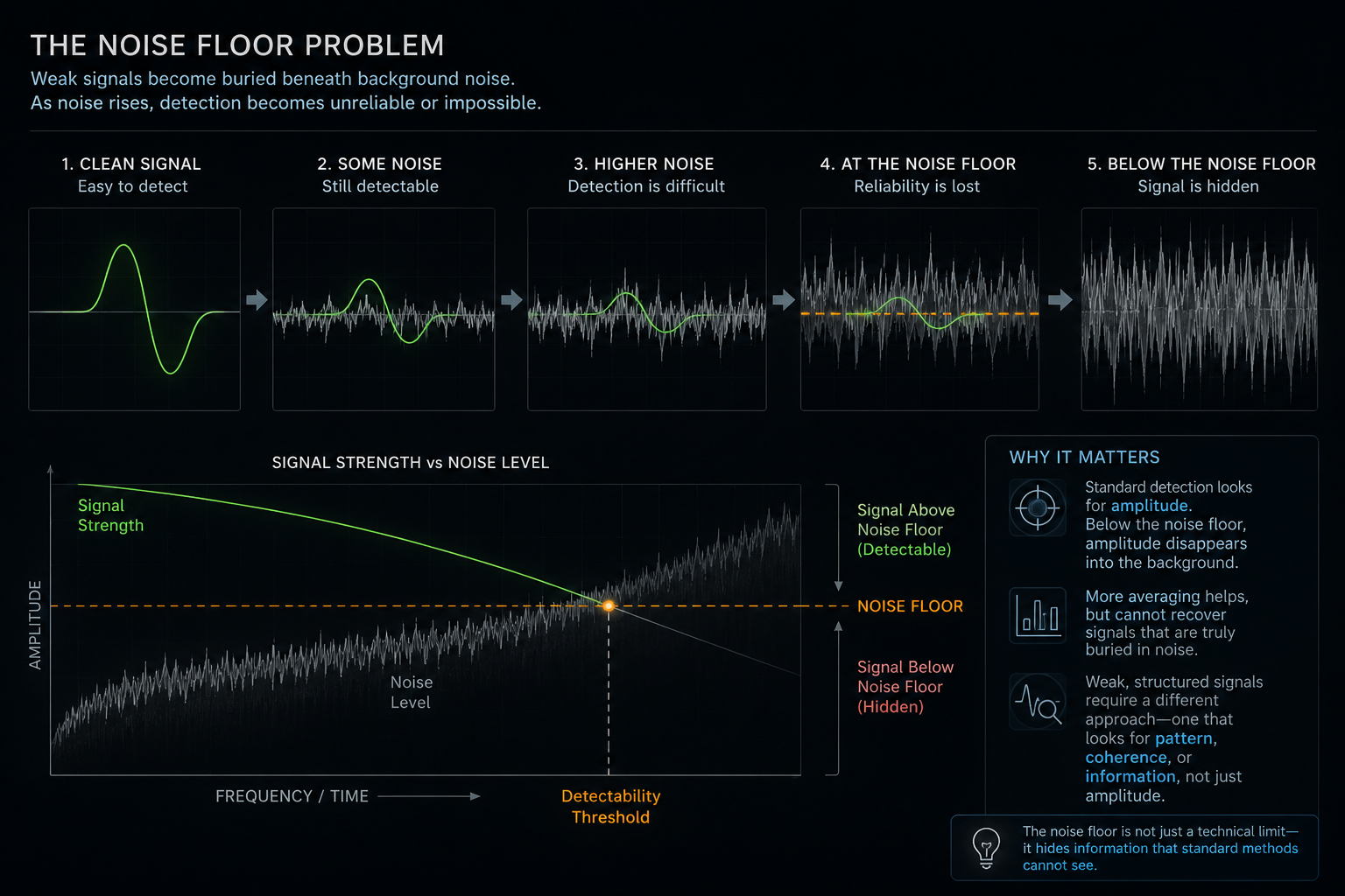
In ordinary signal processing, the noise floor is treated as the point where a receiver can no longer separate useful signal from unwanted variation.
That is a real engineering limit for that receiver.
But it is not automatically a limit of reality.
A receiver can fail before the underlying structure has disappeared. A digital system can output zero because it has no coordinate for what is still present. A signal can fall below an ordinary receiver floor while still leaving coherent structure in the sensor-admitted record.
This is the difference between ordinary DSP and EFSG.
DSP asks whether a declared signal can be recovered through declared receiver coordinates.
EFSG asks whether coherent structure can be recovered from the information admitted by the sensor before ordinary symbolisation destroys it.
Standard DSP View
DSP means digital signal processing.
DSP is used to sample, filter, transform, compress, classify, demodulate and recover useful information from measured data.
It is one of the foundations of modern engineering. Telecoms, radar, sonar, cameras, medical imaging, seismology, audio systems, astronomy, control systems and wireless receivers all depend on it.
A standard DSP system usually begins with a declared task.
Recover the transmitted bit.
Detect the target.
Pick the arrival time.
Identify the frequency.
Classify the event.
Separate signal from noise.
Reduce bit error rate.
Improve signal-to-noise ratio.
To do this, the receiver declares the coordinates it cares about. These may include amplitude, frequency, phase, timing, packet state, threshold crossing, sample value, symbol class or channel estimate.
That is powerful.
But it is also a reduction.
The system keeps what its receiver model can represent. It removes, averages, clips, thresholds, filters, compresses or ignores what falls outside that model.
SNR, BER and the Noise Floor
SNR means signal-to-noise ratio.
It compares the strength of a desired signal with the strength of the surrounding noise.
BER means bit error rate.
It measures how often a digital receiver recovers the wrong bit.
These are essential engineering measures. If the receiver has better separation between signal and noise, the bit error rate usually improves. If the channel becomes noisier, errors usually increase.
Inside ordinary communication systems, this is exactly the right way to think.
The receiver is trying to decide between declared symbols. It needs enough separation to make reliable decisions. If the separation falls too low, the receiver reaches its practical floor.
But the important point is this:
the noise floor is a receiver condition.
It is not automatic proof that the underlying field contains no structure.
Shannon Is Not Wrong
Shannon is not being contradicted.
Shannon describes reliable communication inside a declared channel.
Once the source, channel, bandwidth, signal power, noise model, coding assumptions and receiver variables are declared, Shannon gives the limit of reliable symbolic communication inside that model.
That is not the same as saying all recoverable structure outside the declared model has ceased to exist.
Shannon begins after the channel has been declared.
Davies begins one step earlier.
The Davies question is:
what recoverable structure was excluded, collapsed or named as noise when the channel was declared?
That is why the Shannon limit should be read as a declared-channel boundary. It is not a statement that the sensor-admitted landscape outside the channel is empty.
How DSP Turned Shannon into a Hard Limit
The problem came through the success of DSP.
Digital receivers are quantised. They preserve declared coordinates and discard anything the receiver has no place to store.
If a structure is turbulent, fractal, elastic, harmonic, resonant, boundary-based or time-pathway-dependent, an ordinary DSP receiver may have no coordinate for it.
So the structure appears to vanish.
This is like asking the human eye to see X-rays. The visible-band signal goes to zero, but that does not mean X-rays are absent. It means the receiver has no coordinate for them.
The same thing happens in digital receiver space.
If a structure does not survive sampling, thresholding, binning, filtering, compression, symbolisation or quantisation, it becomes zero inside that receiver output.
The DSP system then appears to self-verify the absence of the structure.
But it has only verified absence inside its own coordinate system.
Shannon did not say the underlying structure goes to zero. His equation does not point to a physical zero of reality. It describes a capacity boundary after the channel has been declared.
The zero is often introduced by the receiver.
The Cost of Digital Quietness
The move from analogue to digital solved a real problem: noise.
Analogue systems are rich, but they are messy. They carry drift, hiss, interference, coupling, phase ambiguity, thermal noise, boundary residue, distortion and unwanted variation.
Digital systems became powerful because they quietened that mess.
Digital is beautifully quiet.
It allows stable computation, clean copying, repeatable storage, error correction, compression, reliable communication and scalable processing.
But the cost of quietness is deletion.
To become quiet, the receiver must decide what counts as signal and what does not. It must choose what to preserve and what to remove.
That removal may delete structure that was irrelevant for the declared task. In that case nothing important is lost.
But it may also delete structure that still carries physical information.
This can include:
phase residue;
micro-timing;
weak coherence;
boundary morphology;
elastic memory;
harmonic relation;
fractal persistence;
turbulent transition structure;
resonant coupling;
time-pathway history;
sub-threshold event-memory.
Digital quietness is not free. It is purchased by reducing analogue complexity.
When the omitted structure matters, a clean digital output can become a clean loss of evidence.
The Omitted-Coordinate Problem
The deepest issue is not whether receivers reduce information. All task-facing receivers reduce information.
The real issue is whether the receiver has a coordinate for the structure that matters.
A digital receiver can sample a fractal-like signal and store finite values, but ordinary quantisation does not automatically preserve scale recurrence or self-similarity.
It can store amplitude values, but that does not automatically preserve phase recurrence.
It can increase bit depth, but that does not automatically preserve elastic memory.
It can increase sampling rate, but that does not automatically preserve boundary morphology.
It can produce a clean symbol, but that does not automatically preserve the path by which the system reached that symbol.
If the receiver has no coordinate for a structure, that structure cannot survive into the final output.
This does not prove the structure was absent.
It proves the receiver output did not carry it.
Receiver Boundary, Not Existence Boundary
A noise floor can feel like an existence boundary because the receiver stops producing useful output.
But it is better understood as a receiver boundary.
The nightclub example makes this simple. Two people standing beside a loudspeaker may not hear each other. Their speech has not stopped existing. The receiver relation has failed.
Jamming works the same way. A jammer does not need to destroy the intended signal. It only needs to raise or distort the receiver environment until the intended signal is no longer recoverable through that receiver’s declared coordinates.
Astronomy uses the positive version. Telescopes are placed in remote, high, dry, dark or radio-quiet environments because the location does not create the astronomical signal. It improves the receiver relation.
The same logic applies to DSP.
A receiver floor means:
this receiver, using this method, in this environment, with this coordinate set, cannot separate the structure reliably.
It does not automatically mean:
there is no structure.
EFSG as a Multi-Optic Receiver
EFSG does not treat the ordinary noise floor as the final boundary.
It treats the receiver-floor region as a mixed region.
That region may contain:
irreducible noise;
instrument artefact;
model mismatch;
nonrecoverable residue;
weak coherent structure;
boundary residue;
phase organisation;
elastic memory;
harmonic relation;
fractal or scale persistence;
cross-channel coherence;
time-pathway information.
Some of that mixture may be useless.
Some may be unrecoverable.
Some may be artefact.
Some may be genuinely incoherent.
But some may be recoverable structure that ordinary DSP grouped with noise because it had no coordinate for it.
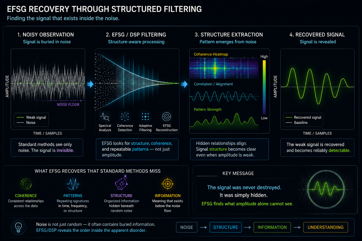
EFSG is designed to test that possibility.
It is not an amplifier. An amplifier raises signal, noise, distortion and error together.
EFSG is a selective coherence recovery method.
It asks:
can coherent structure be recovered from the information admitted by the sensor?
Why Multi-Optic Matters
A single receiver coordinate may miss structure that another coordinate can recover.
This is why EFSG uses multiple optics.
The π optic looks for smooth continuity, drift, slope, curvature and laminar path coherence.
The χ optic looks for boundary behaviour, threshold proximity, intermittency, timing residue, mixing, edge behaviour and cross-channel coherence.
The ψ optic looks for Davies Well closure, balance, coefficient-neutral states and curvature-transition structure.
The H optic looks for harmonic structure, phase relation, subharmonics, overtones and cross-frequency organisation.
The E optic looks for elastic memory, rebound, attenuation, relaxation, reflection, refraction and failed-fold residue.
The F optic looks for fractal or scale-persistent structure across observation windows.
The τ optic looks for time-pathway structure, propagation history, delay, coherence loss and observer-path dependence.
The important point is not the labels.
The important point is that different structures may need different receiver coordinates.
Ordinary DSP asks:
does the declared signal separate from the declared noise?
EFSG asks:
which receiver optic, if any, preserves coherent structure from the admitted record?
Above-Floor vs Recoverable
Standard DSP often divides the world like this:
signal above the floor;
noise below the floor.
EFSG divides it differently:
recoverable coherent structure;
nonrecoverable structure;
irreducible incoherence;
receiver artefact;
model mismatch;
structure not admitted by the sensor.
This is the key difference.
EFSG does not need above-floor and below-floor as its native distinction.
A structure can be weak and still coherent.
A structure can be below a per-sample noise scale and still recoverable through alignment.
A structure can be invisible to one receiver coordinate and visible to another.
A structure can be lost in final symbols but present in raw or lightly reduced data.
So the practical question is not only:
how loud is it?
The practical question is:
does it remain coherent under a valid receiver route?
Below-Floor Coherence
A weak signal may sit below the ordinary per-sample noise scale.
A standard receiver may treat it as below-floor.
But if that weak structure is aligned across many samples, phases, channels, harmonics, paths or time windows, a coherent projection may recover it.
The coherent part adds in the same direction.
The uncorrelated noise tends to average down.
This does not prove all below-floor variation is meaningful.
It proves something narrower:
below one receiver floor does not mean below every possible coherent projection.
That is the opening EFSG uses.
Telecommunications Example
Telecommunications is a clean example because the receiver-side problem is familiar.
A conventional receiver asks:
which symbol was sent?
A boundary-aware receiver asks an earlier question:
what recoverable analogue structure is still present around the symbol decision?
That structure might include phase residue, micro-timing, weak coherence, multipath shape, transition curvature, cross-band recurrence or local persistence near the receiver floor.
If that extra evidence reduces bit error rate, packet error rate, retry burden, required SNR, jitter, latency or keep failure, the gain is receiver-side.
This does not mean EFSG has overridden Shannon inside the same declared channel.
It means EFSG may have preserved recoverable structure before the waveform was reduced into declared Shannon-space variables and final symbol decisions.
If EFSG later projects the recovered structure into a conventional communication channel, the limits of that projected channel apply again.
What EFSG Does Not Claim
EFSG does not claim that all noise contains information.
EFSG does not claim that Shannon is wrong.
EFSG does not claim to recover structure that never entered the sensor-admitted record.
EFSG does not claim that cleaner-looking output is proof.
EFSG does not claim that every boundary is recoverable.
EFSG does not create information.
The correct claim is narrower:
ordinary digital reduction can omit active boundary structure, and EFSG tests whether some of that omitted structure remains recoverable from raw or lightly reduced admitted data.
The Clean Distinction
Shannon defines reliable communication inside a declared channel.
DSP implements a quantised receiver route inside declared coordinates.
The noise floor is the failure point of that receiver route.
Jamming exploits that failure point by overwhelming the receiver relation.
EFSG does not claim the noise floor is unreal.
EFSG says the ordinary noise floor is not an existence boundary.
It asks whether the sensor-admitted record still contains coherent recoverable structure that ordinary DSP did not preserve.
Summary
DSP is powerful because it reduces the analogue world into stable, useful, computable forms.
Shannon is powerful because it defines reliable communication inside a declared channel.
The ordinary noise floor is useful because it tells us where a receiver route stops separating its declared signal from noise.
But none of these proves that the underlying admitted record contains no further recoverable structure.
The noise floor is a receiver boundary.
The Shannon limit is a declared-channel boundary.
DSP is a selected-coordinate recovery route.
EFSG is different because it is a dynamic multi-optic receiver. It does not begin by asking only whether a declared signal is above a fixed floor. It asks whether the admitted record contains coherent recoverable structure that ordinary receiver coordinates did not preserve.
The receiver may stop resolving before the structure stops existing.